PyFunc it! We'll do it Live!

Real-Time Data Preprocessing for Custom Databricks Model Serving Endpoints

When performing real time inference, you rarely get all of the data needed to make your prediction exactly how your model requires it inside the POST request. More commonly, one or both of the following are true:

1. The data received requires significant preprocessing in the form of parsing, encoding, reformatting, etc.

2. The data received is incomplete and must be combined with another data set in order to perform accurate predictions

Today’s blog will focus on the first use case, and we will revisit the second one next quarter. I originally wrote Part 2 using Online Tables, which is still a possibility, but there have been some API changes I want to make sure settle before publishing.

Bill gets frustrated with pre-processing pipelines

The Power of Pipelines

If we have an sklearn model, adding preprocessing steps - even more advanced custom preprocessing classes - is a straightforward task:

import mlflow
import mlflow.sklearn
from sklearn.pipeline import Pipeline
from sklearn.preprocessing import StandardScaler
from sklearn.linear_model import LogisticRegression
from sklearn.datasets import load_iris

# Yes this dataset is simplistic, but we're just proving a point right now
iris = load_iris()
X = iris.data
y = iris.target

# Create the pipeline with whatever preprocessing you may need, Pipeline also accepts custom classes
pipeline = Pipeline([
    ('scaler', StandardScaler()),
    ('model', LogisticRegression())
])

# Start the MLflow run with autologging for even more quality of life features
with mlflow.start_run():
    mlflow.sklearn.autolog()
    pipeline.fit(X, y)

mlflow.end_run()

Not exactly groundbreaking code here. But what if our custom parsing and preprocessing logic was really complex and we wanted to maintain our own separate python scripts for this logic to maintain modularity? What if we wanted to use a model type that doesn't fit nicely into sklearn? Regardless of the specific motivation, the time may come when this pattern will no longer serve our needs. Calling a separate .py file from within a PyFunc Python model and serving the custom pipeline is an extremely powerful and flexible pattern for multipart inference pipelines.

Note: You can still use an sklearn Pipeline for this without using the mlflow.sklearn flavor, because XGBoost provides an sklearn compatible API. I've run the code below both ways, and while you don't have to use a single sklearn package in order to leverage this pattern, it will make for a simpler to follow demo.

Defining a Custom Preprocessing Script

The below .py file contains two relatively simple preprocessing classes, one that flattens nested JSON strings and one that extracts the domain from email addresses.

## custom_transformers.py
## We could break these out, but for simplicity of the demo, I'm just making one external .py file
from sklearn.base import BaseEstimator, TransformerMixin
import pandas as pd

class JSONFlattener(BaseEstimator, TransformerMixin):
    """
    Transforms the DataFrame by flattening the specified JSON column into a tabular format.
    """
    def __init__(self, json_column, record_prefix=''):
        self.json_column = json_column
        self.record_prefix = record_prefix

    def fit(self, X, y=None):
        return self

    def flatten_dict(self, d, parent_key='', sep='.'):
        items = []
        for k, v in d.items():
            new_key = f"{parent_key}{sep}{k}" if parent_key else k
            if isinstance(v, dict):
                items.extend(self.flatten_dict(v, new_key, sep=sep).items())
            else:
                if isinstance(v, list):
                    v = ';'.join(map(str, v))
                items.append((new_key, v))
        return dict(items)

    def transform(self, X):
        X = X.copy()
        flattened = X[self.json_column].apply(lambda x: self.flatten_dict(x, self.record_prefix, sep='.'))
        json_df = pd.DataFrame(flattened.tolist())
        X = X.drop(columns=[self.json_column])
        X = pd.concat([X.reset_index(drop=True), json_df.reset_index(drop=True)], axis=1)
        return X

class EmailDomainExtractor(BaseEstimator, TransformerMixin):
    """
    Transforms the DataFrame by adding a new column 'email_domain' containing the extracted domains.
    """
    def __init__(self, email_column):
        self.email_column = email_column

    def fit(self, X, y=None):
        return self

    def transform(self, X):
        X = X.copy()
        if self.email_column not in X.columns:
            raise ValueError(f"Column '{{self.email_column}}' not found in input data.")
        X['email_domain'] = X[self.email_column].apply(
            lambda x: x.split('@')[-1] if isinstance(x, str) and '@' in x else 'unknown'
        )
        return X

Being a fully self-specified data format, JSON strings are an extremely popular method for sending data over the internet, and in order to suit the wide variety of use cases that leverage JSON, they can get quite complex. Databricks model serving limits the payload of an individual request to 16MB, which a single JSON could hypothetically occupy all of. Needless to say, our two level JSON flattener class is only meant to be a placeholder to showcase a broader pattern.

Now that we have our .py file defined, let's open a notebook in the same folder and turn our cluster on if we don't already have one. For this code I used an r6i.xlarge single node CPU cluster on Databricks ML Runtime 15.4 LTS on AWS, but a rough equivalent in Azure would be the E4s_v4, since both feature 4 vCPUs with 8 GiB of RAM, each powered by Intel Xeon Ice Lake processors. These are both fast and low cost, with the AWS one coming in at 1.02 DBU/hr.

Synthetic Data Generation

To keep the code in this blog fully functional out of the box, we're going to generate some synthetic data using one of my favorite python packages, Faker.

# Note: as we said above, this pattern is not dependent on sklearn Pipelines
%pip install faker==18.11.2
%pip install scikit-learn==1.2.2
%pip install databricks-sdk --upgrade
%pip install mlflow==2.17.0
dbutils.library.restartPython()

# We'll use a non-sklearn ML package for our main model, XGBoost
import pandas as pd
import numpy as np
from faker import Faker
from sklearn.model_selection import train_test_split
from sklearn.pipeline import Pipeline
from sklearn.preprocessing import OneHotEncoder, StandardScaler
from sklearn.compose import ColumnTransformer
from sklearn.impute import SimpleImputer
from sklearn.metrics import classification_report
import mlflow
import mlflow.pyfunc
from mlflow.models.signature import infer_signature
import xgboost as xgb
import joblib
import os
import sys

We'll generate 1,000 rows for now, but you could generate far more if you wanted to experiment with the scalability of your model.

# Faker makes synthetic data generation easy
fake = Faker()
Faker.seed(42)
np.random.seed(42)

def generate_data(num_rows=1000):
    data = []
    for _ in range(num_rows):
        customer_id = fake.unique.uuid4()
        name = fake.name()
        address = {
            'street': fake.street_address(),
            'city': fake.city(),
            'state': fake.state_abbr(),
            'zip_code': fake.zipcode()
        }
        email = fake.email()
        phone_number = fake.phone_number()
        
        transaction = {
            'transaction_id': fake.unique.uuid4(),
            'amount': round(np.random.uniform(10.0, 1000.0), 2),
            'transaction_type': np.random.choice(['online', 'in-store', 'cash withdrawal', 'mobile']),
            'account_age_days': np.random.randint(30, 3650),
            'customer_info': {
                'customer_id': customer_id,
                'name': name,
                'address': address,
                'email': email,
                'phone_number': phone_number
            },
            'fraud': np.random.choice([0, 1], p=[0.95, 0.05])
        }
        data.append(transaction)
    return pd.DataFrame(data)

df = generate_data(num_rows=1000)
display(df.head(5))

---

Short aside: What if my preprocessing logic are other models?

If you had additional ML models in your pipeline, there are a few ways you could incorporate them together depending on the flow pattern of the data. For example, if you have multiple independent processes, then you can use a fan out model where models can process in parallel on their own endpoints, then send those results back to a wrapper model for the final prediction. The pros of this are that you can scale multiple models independently, and if you have multiple heavily duty models, this may be the fastest way to structure things. The cons are that you have more cost, both in terms DBUs (since you have multiple running endpoints) and in terms of overhead latency, since each call from one endpoint to another is going to add ~50ms.

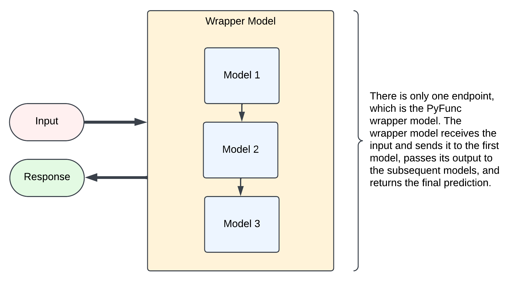
The other option, especially if you have multiple dependent processes, is to wrap the constituent models up in the orchestrator as model artifacts and serve the entire pipeline to a single endpoint. The pros of this are that you save on costs, financially and in overhead latency, and since your model processes are dependent anyway, there is no efficiency loss due to models that could be run in parallel laying idle. The cons are that you need to be more careful in the initial deployment since it's less modularized, but I have some tips to share on that below.

Note that your preprocessing logic being other models does not fundamentally change anything, since a PyFunc model can be really any executable python code that takes X and returns y, you could even host your non-model preprocessing logic on separate endpoints if you wanted to. However, it would be rather unconventional and I can't contrive a scenario where that would be advantageous at the moment.

Multiple Endpoints Version

Single Endpoint Version

In short, when it comes to calling constituent models to obtain intermediate results, you do have some options. However, the most common one is going to be to call those models almost exactly as you would any other preprocessing logic. Great, now back to the main example.

---

Apply Preprocessing Logic from .py Script

Now that we have some data to work with, let's apply those preprocessing functions we defined earlier. All we need to do is specify the path to where our script lives and import our classes as we would any others off PyPI.

# Retrieve the current notebook's full path
notebook_path = dbutils.notebook.entry_point.getDbutils().notebook().getContext().notebookPath().get()
notebook_dir = os.path.dirname(notebook_path)
dbfs_path = '/Workspace' + notebook_dir
# This will come into play when we log the model to mlflow
custom_transformers_path = dbfs_path + '/custom_transformers.py'
from custom_transformers import JSONFlattener, EmailDomainExtractor

# # dbfs_path is already in sys.path but if it weren't we could add it like so:
# if dbfs_path not in sys.path:
#     sys.path.append(dbfs_path)

# Split the dataset
X = df.drop(columns=['fraud', 'transaction_id'])
y = df['fraud']

X_train, X_test, y_train, y_test = train_test_split(
    X, y, test_size=0.2, random_state=42, stratify=y
)

# Define preprocessing steps
numeric_features = ['amount', 'account_age_days']
numeric_transformer = Pipeline(steps=[
    ('imputer', SimpleImputer(strategy='median')),
    ('scaler', StandardScaler())
])

categorical_features = ['transaction_type', 'customer_info.address.state', 'email_domain']
categorical_transformer = Pipeline(steps=[
    ('imputer', SimpleImputer(strategy='constant', fill_value='missing')),
    ('onehot', OneHotEncoder(handle_unknown='ignore', sparse_output=False))
])

preprocessor = Pipeline(steps=[
    ('json_flattener', JSONFlattener(json_column='customer_info', record_prefix='customer_info')),
    ('email_domain_extractor', EmailDomainExtractor(email_column='customer_info.email')),
    ('column_transformer', ColumnTransformer(
        transformers=[
            ('num', numeric_transformer, numeric_features),
            ('cat', categorical_transformer, categorical_features)
        ])
    )
])

Looking good. Remember we don't need to use an sklearn Pipeline for this to work, but we're using it anyway to keep this blog more focused on calling custom preprocessing modules on a live serving endpoint rather than building custom pipelines.

Right, let's train the model! This should take about 30 seconds on our machine with 1,000 rows, but this is far from maxing out our cluster's CPU util or RAM, so it will scale sub-linearly for orders of magnitude more data.

# Fit the preprocessor and transform the data
preprocessor.fit(X_train, y_train)
X_train_processed = preprocessor.transform(X_train)
X_test_processed = preprocessor.transform(X_test)

# Convert processed data to numpy arrays if they are DataFrames
if isinstance(X_train_processed, pd.DataFrame):
    X_train_processed = X_train_processed.values
if isinstance(X_test_processed, pd.DataFrame):
    X_test_processed = X_test_processed.values

# Train the XGBoost model
dtrain = xgb.DMatrix(X_train_processed, label=y_train)
dtest = xgb.DMatrix(X_test_processed, label=y_test)

params = {
    'objective': 'binary:logistic',
    'eval_metric': 'logloss',
    'seed': 42
}

bst = xgb.train(params, dtrain, num_boost_round=100)

# Evaluate the model
y_pred_proba = bst.predict(dtest)
y_pred = (y_pred_proba > 0.5).astype(int)

print("Classification Report:")
print(classification_report(y_test, y_pred, digits=4))

# Prepare artifacts and signature
joblib.dump(preprocessor, "preprocessor.joblib")
bst.save_model("model.xgb")

artifacts = {
    "preprocessor_path": "preprocessor.joblib",
    "model_path": "model.xgb"
}

sample_input = X_train.iloc[:5]
sample_output = bst.predict(xgb.DMatrix(preprocessor.transform(sample_input)))
signature = infer_signature(sample_input, sample_output)

We'll now define the PyFunc wrapper model. Notice that we import our custom package again inside the load_context() function. This ensures all required code is saved to our model's artifacts in MLflow.

# Define the custom PyFunc model
class FraudDetectionModel(mlflow.pyfunc.PythonModel):
    def load_context(self, context):
        import xgboost as xgb
        import joblib
        import pandas as pd
        # Import custom transformers from the installed package
        from custom_transformers import JSONFlattener, EmailDomainExtractor

        # Load the preprocessor and model artifacts
        self.preprocessor = joblib.load(context.artifacts["preprocessor_path"])
        self.booster = xgb.Booster()
        self.booster.load_model(context.artifacts["model_path"])

    def predict(self, context, model_input):
        processed_input = self.preprocessor.transform(model_input)
        if isinstance(processed_input, pd.DataFrame):
            processed_input = processed_input.values
        dmatrix = xgb.DMatrix(processed_input)
        predictions = self.booster.predict(dmatrix)
        return predictions

Additionally, we can prevent possible container build failures by specifying compatible package versions in our predefined conda_env:

conda_env = {
    'name': 'mlflow-env',
    'channels': ['defaults'],
    'dependencies': [
        'python=3.11.0',
        'pip',
        {
            'pip': [
                'mlflow==2.17.0',
                'xgboost==2.0.3',
                'joblib==1.2.0',
                'faker==18.11.2',
                'scikit-learn==1.2.2',
                'numpy==1.23.5',
                'cloudpickle==2.2.1',
            ],
        },
    ],
}

Finally we can log and register the model to MLflow. Two things I want to make note of:

1. The code_path parameter in the log_model() function that we alluded to earlier is crucial for ensuring the model has access to our preprocessing code on the endpoint

2. We alias the latest run as Production and then call @Production at the end of the model_uri in the following cell; we could have omitted this and kept track of version numbers instead, but that's up to you

# Log the model using mlflow.pyfunc
with mlflow.start_run() as run:
    mlflow.pyfunc.log_model(
        artifact_path="model",
        python_model=FraudDetectionModel(),
        artifacts=artifacts,
        conda_env=conda_env,
        code_paths=[custom_transformers_path],
        signature=signature,
        input_example=sample_input
    )
    model_uri = f"runs:/{run.info.run_id}/model"
    registered_model_name = "credit_card_fraud_detection_pyfunc"
    result = mlflow.register_model(
        model_uri=model_uri,
        name=registered_model_name
    )
    print(f"Model registered as {registered_model_name} with version {result.version}")

from mlflow.tracking import MlflowClient

client = MlflowClient()
client.set_registered_model_alias(
    name=registered_model_name,
    alias="Production",
    version=result.version
)

We can check that this functioning as intended by loading the model from MLflow and then running some records through it:

# Load the model using the alias and test predictions
model_uri = f"models:/{registered_model_name}@Production"
loaded_model = mlflow.pyfunc.load_model(model_uri)

new_data = generate_data(num_rows=5)
predictions = loaded_model.predict(new_data)

print("\nPredictions:")
print(predictions)

The above shows that this works in the notebook environment, but a common problem data scientists face is something working in the notebook but failing on the endpoint. We can dramatically speed up the process of testing dependency agreements and other environment variables by using the mlflow.models.predict() functionality too. The difference between this and load_model() may not seem obvious at first glance, especially because the documentation doesn't fully explain this important distinction, but mlflow.models.predict() builds a lightweight virtual environment based on the conda_env we specified earlier, making it a much closer proxy for the endpoint than load_model() which uses the notebook's existing environment. You'll notice mlflow.models.predict() takes about 5-10x longer than load_model(), but a minute here may save you hours of iterative development if your alternative is waiting to see if your endpoint environment is valid!

In November 2024, the Databricks documentation for mlflow.models.predict() were updated to better explain this.

import os
import json

# Define temporary output path
output_path = "/tmp/mlflow_predictions.json"

# This is a much better test than loaded_model.predict()
mlflow.models.predict(model_uri, new_data, output_path=output_path)

# Read predictions from the output file
with open(output_path, "r") as f:
    predictions = json.load(f)

mlflow.end_run()

And we’re done! If you’ve made it this far, I applaud you. Let’s quickly recap what we’ve done here:

• Demonstrated how to reference an external script within a PyFunc model

  • In the form of a data preprocessing pipeline for real-time inference

• Implemented an end-to-end fraud detection pipeline

  • With a non-sklearn model and our custom preprocessing

• Properly packaged, logged, and registered our custom code with MLflow

  • Tested both in the notebook environment and a simulated deployment environment

Happy coding!