

Have you noticed unexpected results from Databricks Vector Search’s similarity_search? If you’re coming from a cosine similarity background, the scores might seem puzzlingly misaligned with your expectations. In this blog, we’ll dive deep into why this happens, explain the key differences between similarity metrics, and provide a solution to bridge this gap.
Cosine Similarity
Let’s start with a quick refresher on cosine similarity. The cosine similarity between two vectors a and b defined as:
Geometric Interpretation
Cosine similarity gives us a clear geometric intuition for vector similarity by measuring the angle between them in vector space. If two vectors point in the same direction, their cosine similarity is 1; if they are orthogonal (at 90°), it is 0; and if they point in opposite directions, it is –1. This works because cosine similarity is simply the cosine of the angle between them in their vector space.
Think of it like comparing the orientation of arrows: two arrows pointing in the same direction, no matter how long, are perfectly aligned (cosine = 1), while arrows at right angles share no alignment (cosine = 0), and arrows pointing in opposite directions are fully misaligned (cosine = –1). Unlike Euclidean distance, which can be influenced by the length of the vectors, cosine similarity purely reflects alignment, making it especially useful in high-dimensional spaces where magnitude may vary but direction carries semantic meaning.
Here is a sample implementation
import numpy as np

def cosine_similarity(a, b):
    a = np.array(a)
    b = np.array(b)
    dot_product = np.dot(a, b)
    norm_a = np.linalg.norm(a)
    norm_b = np.linalg.norm(b)
    return dot_product / (norm_a * norm_b)
In practice, many of us rely on the scikit-learn implementation.
import numpy as np
from sklearn.metrics.pairwise import cosine_similarity

# Example vectors
a = np.array([1, 2, 3])
b = np.array([4, 5, 6])

# Reshape for sklearn (expects 2D arrays)
similarity = cosine_similarity(a.reshape(1, -1), b.reshape(1, -1))[0][0]
Interestingly, when the input vectors are normalized to unit length so that
cosine similarity reduces to a simple dot product:
In cases where we want to set a bound, cosine_sim ∈ [0, 1], we may apply a linear transformation such as
which preserves order, and simply squashes the outputs of your cosine similarity function into the new range. This can be very beneficial in circumstances where your similarity scores are used as intermediate inputs to downstream models that have strict boundary requirements, or are sensitive to negative values.
Another variation that you may have seen before is the cosine distance, which is just 1 − cosine_sim. This is often used in conjunction with the other transformations, but provides an interpretation based on the distance (smaller is closer) instead of the alignment (higher is closer).
Databricks’ Similarity Computation
It is possible that you have noticed that neither of these methods produce the scores that you see when you perform a similarity_search using the Databricks VectorSearchIndex class. In contrast, from the Official Databricks Documentation, we can see that databricks uses the following formula to compute similarity:
Where
While this formula relies on the euclidean distance, you can see that it is not just the euclidean distance. In contrast to cosine similarity, which compares direction, this score relies on a linear transformation of Euclidean distance, which compares position. If the vectors are not normalized, the algorithm sensitive to both the magnitude and alignment of the vectors. For example:
Two vectors pointing in the same direction but with very different lengths may have high cosine similarity but large Euclidean distance.
Conversely, two vectors that are numerically close (in terms of component values) but not aligned may have small Euclidean distance but low cosine similarity.
This positional sensitivity makes the score potentially misleading in semantic spaces (like embeddings) where direction is more meaningful than length.
For clarity, here’s the Databricks similarity scoring function referenced in our examples:
def euclidean_distance(q, x):
    """Calculate Euclidean distance between vectors q and x"""
    q = np.array(q)
    x = np.array(x)
    return np.linalg.norm(q - x)

def databricks_similarity_score(q, x):
    """similarity score based on the formula: 1 / (1 + dist(q, x)^2)"""
    distance = euclidean_distance(q, x)
    return 1 / (1 + distance ** 2)
Side Note - Hybrid Similarity Score
There is an additional step for providing the score if a hybrid search, if using the query_type='HYBRID' argument when calling the VectorSearchIndex.similarity_search method, a composite BM25 Keyword and Vector similarity is used. This score
relies on an algorithm called Reciprocal Rank Fusion (RRF), and aggregates rankings from several sources into a single, ranking. For more detailed information about this, please see Ref (1).
Vector Normalization
Vector normalization rescales a vector to have unit length (i.e., L2 norm of 1). This process preserves the vector’s direction while standardizing its magnitude, which is crucial for reliable similarity comparisons.
Given a vector a, its normalized form is:
Normalization essentially projects all vectors onto the unit hypersphere in n-dimensional space, allowing us to compare them purely by their direction and eliminating magnitude differences that can distort similarity measures.
Here is the vanilla python implementation
import numpy as np

def l2_normalize(vector):
    vector = np.array(vector)
    norm = np.linalg.norm(vector)
    if norm == 0:
        return vector  # Avoid division by zero
    return vector / norm
Though in practice, most of us rely on the scikit learn implementation
from sklearn.preprocessing import normalize
import numpy as np

# Each row will be treated as a separate vector
X = np.array([[1, 2, 3], [4, 5, 6]])

# Normalize along rows (axis=1)
X_normalized = normalize(X, norm='l2', axis=1)
Why Normalize?
So, why is normalization so important?
This sketch illustrates the geometric difference between cosine similarity and the Databricks similarity score, which is derived from squared Euclidean distance.
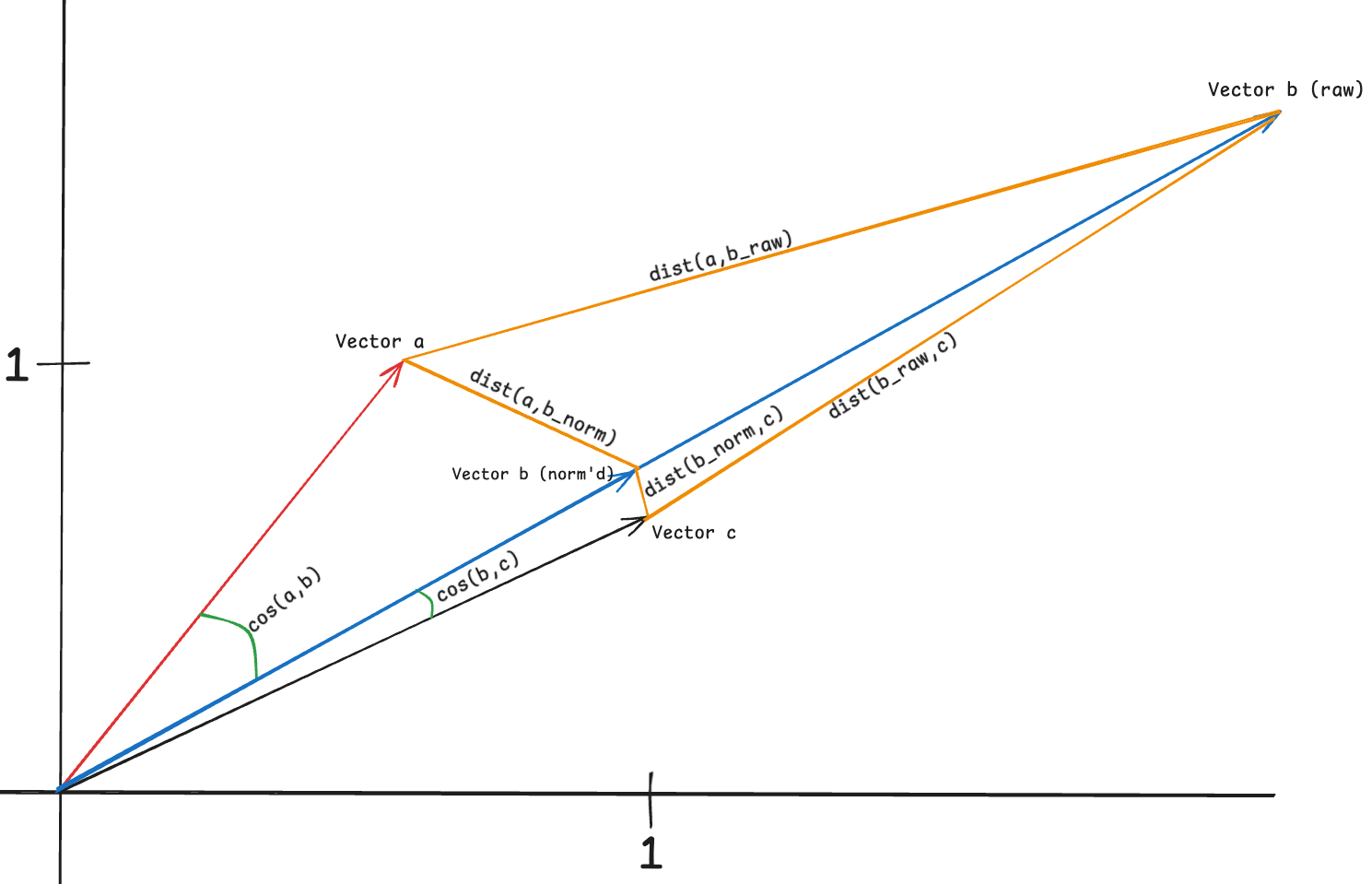
The green angles between vectors (e.g., cos(a, b) and cos(b, c)) represent cosine similarity, which depends purely on direction. In contrast, the orange segments represent Euclidean distances between vector tips — and since the Databricks score is computed as a linear transformation of the distance, these distances directly influence the similarity score.
When embeddings are not normalized, the magnitude of the vectors affects the result. Even though Vector b (raw) is directionally aligned with Vector a, its large magnitude causes the straight-line distance dist(a, b_raw) to be quite large — leading to a low Databricks score. At the same time, Vector c, which is closer in space but less aligned in direction, will have a smaller Euclidean distance to a, and therefore a higher similarity score under the Databricks formula. This misrepresents their true semantic similarity if you were expecting cosine-like behavior.
This is why normalization is essential: when all vectors are normalized (as with Vector b (norm’d)), the Databricks similarity score becomes a function of angle alone — effectively mirroring cosine similarity.
While normalization offers a range of benefits — like simplifying cosine similarity computation, removing scale bias, and improving behavior in clustering — the key reason we normalize embedding vectors in Databricks Vector Search is to ensure rank-order equivalence to cosine similarity.
Rank-Order Equivalence
Rank-Order Equivalence: When vectors are normalized to unit length, the ranking of results by L2 distance matches the ranking by cosine similarity, even though the actual numerical score values differ.
When all vectors are normalized to unit length, the rank order of L2 distances becomes equal to the rank order of cosine similarities. This allows you to take advantage of fast approximate L2 search while still reasoning about results as if you’re using cosine similarity.
One misconception is that this relationship is numerically equal (similarity scores will be exactly equal between the two). This is not the case, and they can be very different in some cases. However, if you consider only their order in the ranking, that relationship is preserved, assuming embeddings are normalized.
Model-Specific Note: GTE vs. BGE
The BGE (BAAI General Embedding) model produces normalized embeddings by default.
The GTE (General Text Embedding) model does not produce normalized embeddings out of the box.
Other External models may or may not provide normalized embeddings, so ensure that you check this if using external models.
If you’re using embeddings from a model that are not normalized by default in Databricks Vector Search, it is strongly recommended to normalize them before indexing. This can be done with any L2 normalization function (like sklearn.preprocessing.normalize). Additionally, you must apply the same normalization strategy to your query vectors at retrieval time that you used when building the index. In other words, if you normalize during indexing, you must also normalize your queries, and if you don’t, then skip it at query time too.
Failing to match the normalization behavior between index and query time will result in invalid similarity comparisons and misleading results. Consistency is key to ensuring your search results are meaningful and accurate.
As demonstrated in these examples, when all vectors are properly normalized, the ranking order is identical between cosine similarity and Databricks similarity scores. This confirms the rank-order equivalence principle, which is crucial for reliable vector search.
Examples
Consider the following code:
import numpy as np
from sklearn.metrics.pairwise import cosine_similarity, euclidean_distances
from sklearn.preprocessing import normalize

# Example vectors
a = np.array([1.0, 0.0])
b = np.array([0.0, 1.0])
c = np.array([1.0, 1.0])
d = np.array([0.2, 0.8])

cos_distance = cosine_similarity(a.reshape(1, -1), b.reshape(1, -1))[0][0]
db_distance = get_databricks_similarity_score(a, b)

print(f"cosine(a,b): {cos_distance}")
print(f"db_distance(a,b): {db_distance}")

vectors = {
    "a": a,
    "b": b,
    "c": c,
}

cosine_scores = {}
db_scores = {}

for name, vec in vectors.items():
    cosine_scores[name] = cosine_similarity(d.reshape(1, -1), vec.reshape(1, -1))[0][0]
    db_scores[name] = get_databricks_similarity_score(d, vec)

cosine_ranking = sorted(cosine_scores.items(), key=lambda x: x[1], reverse=True)
db_ranking = sorted(db_scores.items(), key=lambda x: x[1], reverse=True)

print("\n--- Pairwise Similarity to 'd' ---")
print("Cosine Similarity Scores:")
for name, score in cosine_ranking:
    print(f"{name}: {score:.4f}")

print("\nDatabricks (L2-based) Similarity Scores:")
for name, score in db_ranking:
    print(f"{name}: {score:.4f}")

print("\nCosine Similarity Ranking:", [name for name, _ in cosine_ranking])
print("Databricks Similarity Ranking:", [name for name, _ in db_ranking])
Which will produce the following outputs
cosine(a,b): 0.0
db_distance(a,b): 0.33333333333333326

--- Pairwise Similarity to 'd' ---
Cosine Similarity Scores:
b: 0.9701
c: 0.8575
a: 0.2425

Databricks (L2-based) Similarity Scores:
b: 0.9259
c: 0.5952
a: 0.4386

Cosine Similarity Ranking: ['b', 'c', 'a']
Databricks Similarity Ranking: ['b', 'c', 'a']
Notice that while the numerical scores are much different, the rankings are
preserved. This is because the input vectors in the example are all normalized by definition.
Lets try that again, but this time, we will use arbitrary vectors that are not normalized.
# Define non-normalized versions of the same vectors
a_raw = np.array([2.0, 0.0])
b_raw = np.array([0.0, 3.0])
c_raw = np.array([5.0, 5.0])
d_raw = np.array([1.0, 4.0])
Below, we can see that the results no longer respect rank-order equivalence
--- Pairwise Similarity to 'd_raw' (Non-Normalized Vectors) ---
Cosine Similarity Scores (Non-Normalized):
b_raw: 0.9701
c_raw: 0.8575
a_raw: 0.2425

Databricks (L2-based) Similarity Scores (Non-Normalized):
b_raw: 0.3333
a_raw: 0.0556
c_raw: 0.0556

Cosine Similarity Ranking (Non-Normalized): ['b_raw', 'c_raw', 'a_raw']
Databricks Similarity Ranking (Non-Normalized): ['b_raw', 'a_raw', 'c_raw']
Notice how the rankings diverged when using non-normalized vectors! Vector c_raw dropped from second to last place in the Databricks ranking despite main- taining its cosine position. This clearly demonstrates why proper normalization is essential when working with Databricks Vector Search if you want results that align with semantic expectations.
And, if we normalize the raw vectors above
a_norm = normalize(a_raw.reshape(1,-1))
b_norm = normalize(b_raw.reshape(1,-1))
c_norm = normalize(c_raw.reshape(1,-1))
d_norm = normalize(d_raw.reshape(1,-1))
and recheck them, we can see that the relationship is again preserved
--- Pairwise Similarity to 'd_norm' (Normalized Vectors) ---
Cosine Similarity Scores (After Normalization):
b_norm: 0.9701
c_norm: 0.8575
a_norm: 0.2425

Databricks (L2-based) Similarity Scores (After Normalization):
b_norm: 0.9436
c_norm: 0.7782
a_norm: 0.3976

Cosine Similarity Ranking (Normalized): ['b_norm', 'c_norm', 'a_norm']
Databricks Similarity Ranking (Normalized): ['b_norm', 'c_norm', 'a_norm']
A Bridge Between These Metrics???
Suppose that you require the interpretability of actual cosine similarity scores. For example, you want to apply semantic thresholds, visualize search relevance, or feed scores into a downstream model. But you still want to take advantage of the fast, scalable L2-based indexing provided by Databricks Vector Search.
What do you do?
The Good News
If your embedding vectors are L2-normalized before indexing, and your query vectors are also normalized at retrieval time, there’s a direct mathematical relationship between the Databricks similarity score and cosine similarity. That means you can recover cosine similarity — exactly — from the score that Databricks returns.
The Algebra
The following derivation shows how to convert between Databricks similarity scores and cosine similarity. If you’re primarily interested in the practical application, feel free to skip to the “Final Formula” section.
Let’s recall how Databricks computes similarity:
If both vectors, a and b are L2-normalized, then:
Plug that into the Databricks score:
Now solve for cos(θ) from the Databricks score:
Invert both sides:
Move terms:
Finally, divide both sides and simplify:
Final Formula
Assuming normalized vectors:
Sample Implementation
Lets implement this in vanilla python so we can test it out!
def cosine_from_databricks_score(score):
    """Convert Databricks similarity to cosine similarity"""
    return 1 - 0.5 * (1 / score - 1)
Experimentation
from sklearn.metrics.pairwise import cosine_similarity
from sklearn.preprocessing import normalize

# Define example vectors
a = np.array([1.0, 2.0, 3.0])
b = np.array([4.0, 5.0, 6.0])

# Normalize the vectors
a_norm = normalize(a.reshape(1, -1))[0]
b_norm = normalize(b.reshape(1, -1))[0]

# Compute cosine similarity directly
cosine_true = cosine_similarity(a_norm.reshape(1, -1), b_norm.reshape(1, -1))[0][0]

# Compute Databricks-style similarity score implemented eariler
db_score = databricks_similarity_score(a_norm, b_norm)

# Convert back to cosine similarity
cosine_reconstructed = cosine_from_databricks_score(db_score)

print(f"True cosine similarity:        {cosine_true:.8f}")
print(f"Databricks score:              {db_score:.8f}")
print(f"Reconstructed cosine from DB:  {cosine_reconstructed:.8f}")
Which produces the following output
True cosine similarity:        0.97463185
Databricks score:              0.95171357
Reconstructed cosine from DB:  0.97463185
Why This Is Precise
This formula is algebraically exact — not an approximation — under the key assumption that both vectors are normalized. In that case, the relationship between cosine similarity and L2 distance becomes a clean geometric identity, and the Databricks score becomes a transformed version of cosine similarity.
The only sources of deviation would be:
Numerical precision issues (e.g., in high dimensions)
Vectors not being normalized
As long as normalization is handled properly, this conversion is 100% faithful
to what cosine similarity would return.
Why You Might Want to Use It
Recover interpretability: You get the familiar cosine scale of –1 to 1, or optionally [0, 1] if re-bounded
Apply thresholds: Use well-understood semantic cutoffs like 0.75 or 0.9
Post-process top-k results: After retrieving candidates from the index, re-score using this formula and sort/filter as needed
Blend with other cosine-based systems: Helps when migrating to or integrating with other platforms that rely on cosine similarity
In short: this gives you the best of both worlds — the performance of L2-based search with the intuitive power of cosine similarity.
Conclusion
So there you have it! The mystery of Databricks Vector Search similarity scoring demystified. Let’s recap what we’ve learned on this mathematical journey:
Cosine similarity focuses on the alignment (direction) of vectors, making it ideal for semantic similarity in embedding spaces.
Databricks similarity measures positional differences stemming from reliance on L2, straight line, Euclidean distance.
Normalization is the critical bridge between these two worlds — when vectors are normalized, the rank order of results becomes equivalent between cosine similarity and Databricks’ scoring system.
If you need actual cosine similarity values (not just rankings), you can precisely recover them from Databricks scores using our conversion formula
This understanding gives you the best of both worlds: the performance and scale of Databricks Vector Search with the interpretability and familiarity of cosine similarity. No more scratching your head when similarity scores don’t match!
Remember that consistency is key — if you normalize your vectors during indexing (which you absolutely should for most embedding models), make sure to apply the same normalization to your query vectors at search time. And if you’re working with models like GTE that don’t normalize by default, take that extra step to ensure your embeddings live on the unit sphere.
Armed with these insights, you can now confidently build sophisticated vector search applications in Databricks that behave exactly as you expect them to. Happy searching!
Sources: (1) Cormack, G. V., Clarke, C. L., & Buettcher, S. (2009, July). Reciprocal rank fusion outperforms condorcet and individual rank learning methods. In Proceedings of the 32nd international ACM SIGIR conference on Research and development in information retrieval (pp. 758-759).