A practical guide to Decision Models on Databricks

Decision Models, System One Models, Jev-like Models

A practical guide to decision models on Databricks

Decision models classify, route and score text with a probability for every possible answer. This post explains when to use them instead of a general LLM, and how to choose the right option on Databricks for each of your use cases.

Summary

• If your task is a choice from a known set of answers, a decision model is usually the better tool. It returns a probability for every answer without generating any free text, which makes it fast and inexpensive at scale, and lets you automate the cases it is confident about while routing the rest to a fallback.

• Start with a built-in decision model on Databricks, such as ai_decide for tables or the System One API for applications, which works on most choice tasks without training. Move to a model fine-tuned on your own labels when you need the highest accuracy or the lowest cost per decision on a label set that rarely changes.

• Calibrate whichever model you choose, and measure how much of your traffic it can handle on its own. A few hundred labeled examples are enough to set a confidence threshold that keeps errors within your budget, and the share of decisions the model makes above that threshold is what turns accuracy into saved work.

Much of the AI in production makes decisions

A large share of the AI running in production today makes decisions. For instance, it routes support tickets to the right team, flags transactions for review, checks whether a claim includes every required document, or estimates how urgent a message is. Each of these tasks is a choice from a known set of answers, and many of them are made thousands or millions of times a day.

A general LLM can make these choices, and it often gets them right. It answers in free text, however, so you have to parse the response, handle the occasional answer that is not on your list, and work without a reliable measure of how certain the model is. You also pay for every token it generates, which adds up quickly at high volume. In short, a general LLM becomes slow and expensive at scale, and hard to automate safely.

Decision models are designed for exactly this kind of work. In this post, we explain what they are, walk through the options on Databricks, and show how to choose between them.

What is a decision model?

A decision model takes a piece of text, a question and the list of allowed answers, and returns a probability for each answer. In LLM-based decision models, those probabilities come from a single forward pass that produces one output token, while encoder decision models score the options directly. Either way, there is no free text to parse and the answer is always one of your options.

In the example below, an insurer routes incoming emails to the right team. The model receives the question, four options and the email, and returns a probability for each option. With 0.94 on auto claims, the email can be routed automatically, while an email with no clear winner would go to the fallback.

Question: Which team should handle this email?
A: Auto claims
B: Home claims
C: Billing
D: None of these
Email: Someone reversed into my car in a parking lot yesterday. How do I file a claim?

Model output (one token): A 0.94, B 0.01, C 0.02, D 0.03

The model responded with a high score of 0.94 for auto claims, so this email can be routed straight to that team. An email with no clear winner would instead go to the fallback.

The short labels are what make this possible. Each option is given a label, such as A, B or C, that the model’s tokenizer treats as a single token. One forward pass then scores every option at once, and the probabilities are normalized over exactly the options you provided. Reading the probabilities of option labels in this way is a well-established technique, widely used to evaluate LLMs on multiple-choice questions. Single letters cover up to 26 options; for longer lists, a model can be fine-tuned to answer with two-letter codes such as AA and AB, as we describe later.

Why generating a single token matters

Choosing an answer from a list does not require writing a paragraph. A chat model that explains its reasoning can generate tens or hundreds of tokens for every decision, and generating tokens is usually the slowest and most expensive part of running an LLM. An LLM-based decision model generates a single token. Most of its work goes into reading the prompt, which is much faster, and the part of the prompt that stays the same across requests can be cached.

Large general LLMs can still be very capable classifiers, especially when they reason through a difficult case before answering. Where decision models pull ahead is speed and cost at scale. A small LLM that writes only the label is faster than a reasoning model, but it still generates several tokens and gives no probability for each option. In our tests, a reasoning model took between 0.7 and 1.5 seconds per decision, while decision models answered in a fraction of that, roughly a tenth of a second through a hosted API and tens of milliseconds on dedicated Databricks GPU compute. At a few hundred decisions a day, that difference hardly matters. At millions a day, it determines how many GPUs you need, how long a nightly job runs and what each decision costs.

Why the probability matters

Because you get a probability for every answer, you can let the model act on its own when it is confident and route the remaining cases to a fallback. That fallback might be a human reviewer, a larger and more capable model, or a slower process that gathers more information. How much of your traffic the model can handle on its own, at an error rate you are willing to accept, is where most of the business value comes from.

Designing the question

It is recommended to keep the decision options mutually exclusive, and to add a short description to any option whose name could be read more than one way. It is also a best practice to include a “none of these” option, because real traffic always contains inputs that fit nothing on your list. When more than one answer can apply at once, such as several product tags on the same review, ask a separate yes or no question for each one, or use a classifier that can return several labels. When you need several answers about the same text, such as an intent and an urgency score, ask them in a single call so the model reads the text only once.

Your options on Databricks

Your options fall into two major groups, depending on whether you need something you can use immediately or a model trained for a particular task.

• Generic options require no training and can answer any question over any set of options.

• Task-specific models, by contrast, are trained on your own labeled examples to handle one defined task.

Some of the features below are in Beta or Preview, so check the linked documentation for their current status and availability in your region.

Built-in options with nothing to deploy

The first three options are AI Functions that you call from SQL, and you can also call ai_decide and ai_classify from an application through the AI Functions REST API. They run directly on your governed Delta tables, where your data already lives, and Databricks manages the parallelism, retries and scaling for you. That makes them a natural way to score millions or billions of rows in a scheduled job or a Lakeflow pipeline, without moving data or managing any infrastructure.

ai_decide brings decision models to SQL. You can ask three kinds of questions about each row: a choice among up to 255 labels, a yes or no question, or a score on an ordered scale. For each question it returns a probability for every allowed answer, and several questions about the same row are answered in one call, which keeps the cost of extra questions low. It is tuned for speed and suits quick decisions such as routing requests, triaging tickets, flagging events that need attention and deciding when a case should go to a larger model. Here’s the insurer example over a table of emails:

SELECT
  email_id,
  decision:response.answers.team.choice::string AS team,
  decision:response.answers.team.confidence::double AS confidence
FROM (
  SELECT
    email_id,
    ai_decide(
      body,
      ‘{
        “team”: {
          “type”: “choice”,
          “instructions”: “Which team should handle this email?”,
          “criteria”: {
            “auto_claims”: “Claims about cars and other vehicles”,
            “home_claims”: “Claims about homes and property”,
            “billing”: “Payments, invoices and premiums”,
            “none”: “None of these”
          }
        }
      }’
    ) AS decision
  FROM main.claims.inbound_emails
)

For the parking-lot email, the above query returned auto_claims with a confidence of 0.98 in our test. The full result also includes probabilities, with a probability for each label. To ask more questions about the same email, such as its urgency on a score scale, add them to the same JSON object.

ai_classify assigns each row one or more labels from a list of up to 500 that you provide. You can add a description to each label and instructions for the task, and version 2.1 also returns a confidence score for each chosen label. It is the quickest way to label a table, with a single line of SQL, no model to select and no infrastructure to manage, and it is a strong choice for large or detailed taxonomies and for long or complex documents. When you need a probability for every option, or several quick decisions about each row, ai_decide is the better fit.

ai_query with a response format sends each row, together with your own prompt, to an LLM on Databricks’ Foundation Model APIs (or an external model or your own serving endpoint), and the responseFormat argument restricts the answer to your list of labels. It is the right choice when you want to add custom instructions or domain context to the prompt, extract other fields along with the label, or use a particular model. For large batch jobs, Databricks recommends its hosted foundation models. Speed and cost per row depend on the model you choose: a general LLM that writes out its answer usually takes longer and costs more per row than a decision model, which is the trade-off for that flexibility.

The System One API is the option for real-time decisions. A single REST call answers one or more yes or no, choice or score questions about the same input and returns a probability for each answer. Because the questions and options are sent with each request, they can change from one call to the next, which suits applications and agents. Response time depends on the model, the input and the request load. Two models are available:

• OpenJev, an open decision model based on Qwen3.5 and hosted by Databricks.

• Jev, a proprietary decision model hosted by TypeSafe AI and served through Unity Gateway. An account admin may need to enable access to it, and TypeSafe’s terms govern its use.

Both use the same API, so you can compare them on your own data for accuracy, latency, cost and data-handling requirements.

Open models you host on Databricks, without training

Open decision models (for example, Clef-Flash from Cloudflare, d1-3B from Liquid AI, Kev-4B and others) are open checkpoints, available on Hugging Face, that have been trained specifically to answer decision questions. You run them with an inference engine such as vLLM on Databricks GPU compute, either on AI Runtime, Databricks’ serverless GPU compute, which we recommend, or on GPU-enabled classic compute, and call them through the same System One API, which gives you a decision API on weights you control. Before you rely on one, check that its license allows commercial use by your organization, since some open decision models restrict it. Also check whether the model may have seen your evaluation data during training.

Any open LLM can also be turned into a decision model without training. You place the options in the prompt and read the model’s probabilities for the option labels. LLMs tend to favor certain positions in a list, so it helps to remove that bias, for example by rotating the order of the options and averaging the results. This gives you a quick baseline on a model you may already be running.

Models trained on your labels

When you have labeled examples, there are four common ways to train a model on them. They differ in what the model learns and in how flexible it remains when your labels change.

• Fine-tune a decision LLM. A small LLM is trained, typically with LoRA, to answer with the label of the correct option. The options stay in the prompt, so one model can answer several questions or serve several related tasks, and you can serve and calibrate it in the same way as a generic decision model. It runs well with vLLM on Model Serving through custom LLM serving.

• Fine-tune an encoder classifier. A BERT-style encoder such as ModernBERT is trained with an output layer for your labels. It is small, fast and inexpensive to serve as a custom model on Model Serving, packaged with MLflow, on either CPU or GPU, but it is tied to its label set, so adding a label means training it again.

• Fine-tune an encoder decision model. A model such as Laya reads the options as part of its input, much as an LLM does, while keeping the speed of an encoder. It needs fine-tuning on your task to perform well.

• Train a head on a frozen LLM. Only a linear layer is fitted on top of the LLM’s internal representation of the text. This needs no fine-tuning run and, once the features have been extracted, can be refitted in seconds when your taxonomy changes, but every decision still runs the full LLM, so serving it costs about as much as serving a fine-tuned decision LLM.

If you do not have labels yet, a common approach is to have a strong reasoning LLM, for example through ai_query, label a sample of real inputs, and to have subject-matter experts review a share of those labels. Make sure the sample covers every label and the hard, borderline cases, and keep a set labeled by experts for testing and calibration, so that you measure the model against human judgment rather than against another model’s answers.

In our tests, we fine-tuned Qwen3 and Qwen3.5 models from 0.6B to 4B parameters with LoRA, which took about 15 minutes on a single H100 GPU with about 10,000 labeled examples. We also trained a ModernBERT encoder, Laya and a linear head on a frozen Qwen3.5-4B. The LoRA models and ModernBERT reached between 90 and 93% accuracy and the frozen head 90%. Laya reached 84% with our default training settings, so it likely has room to improve with tuning. You can run all of this training on AI Runtime.

Five factors that drive cost and quality

The five factors below apply to most decision tasks, whatever your data. Where it is useful, we add evidence from a quick benchmark we ran on Banking77, in which customer messages are routed to one of 77 intents. Your own numbers will differ with your data and your use case, so treat ours as illustrations rather than targets, and run the same comparison on a sample of your own.

1. Training for the task decides how far accuracy can go

A fine-tuned model has learned your specific task: your labels, the way your users phrase things, and where the boundary falls between labels that sound alike. A generic decision model has only the question and the option names to work from, for whatever task you give it. That flexibility is what lets you start right away, and it is also why a model trained for one task usually goes further on that task. On our benchmark, the generic options reached up to about 85% accuracy with no labels at all, while the trained models reached 90 to 93%.

The trade-off is that a fine-tuned model is tied to what it learned. Adding a label, changing a definition or starting a new use case usually means collecting new labels and training again. Fine-tuning pays off when the label set is stable and either the volume is high or you need the highest accuracy you can get.

2. Calibration decides how much you can automate

When a model reports 90% confidence, it should be right about 90% of the time, but raw model probabilities often fall short of that. The usual fix has two steps. First, fit a single temperature on a few hundred labeled examples that the model has not seen; this rescales every confidence score without changing which answer wins. Then choose the lowest confidence threshold at which errors stay within your budget. For options that return a single confidence score rather than a probability for every answer, such as ai_classify, skip the temperature and set the threshold directly on your labeled examples. A reliability plot or the Brier score will show whether the calibration worked, which accuracy alone cannot tell you. In our benchmark, with 500 labeled examples and a 5% error budget, the fine-tuned model handled about 95% of messages on its own.

The chart below shows the full trade-off. The tighter your error budget, the less you can automate, and on this measure the gap between trained and untrained models is much wider than on raw accuracy. At a 5% budget, both fine-tuned models automate about 96 to 97% of messages, while the generic decision model automates about two-thirds. At 2%, the generic model drops to about a third, and the fine-tuned models still handle more than 85%.

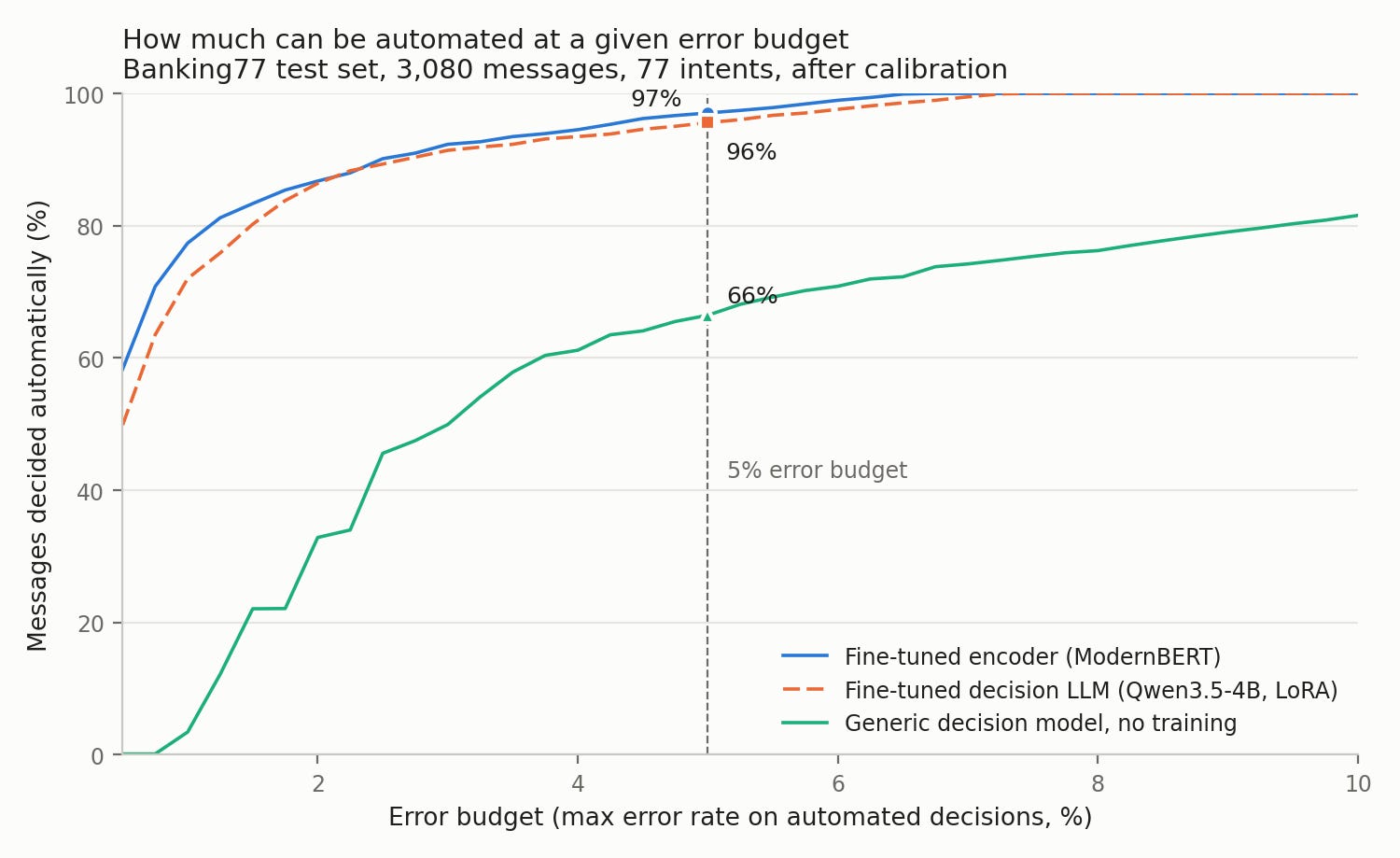
Banking77 test set (3,080 messages), after temperature calibration. Each point uses the best threshold for that budget on the test set, so it’s a little optimistic compared with a threshold chosen on held-out labels.

Store the temperature, the threshold and the fallback together with the model, and refit them when the model or your traffic changes. In production, track three numbers: the share of decisions made automatically, the error rate on that share, and the cost per decision.

3. Your label set decides between an encoder and a decision LLM

If your label set is fixed and you have thousands of examples, a fine-tuned encoder is the natural starting point. Because it is many times smaller than even a small LLM, it usually has lower latency, much higher throughput and a much lower cost per decision on the same hardware. On our benchmark it was also the most accurate, and about six times cheaper per decision than our most efficient decision LLMs. On other tasks, a fine-tuned LLM sometimes comes out ahead, so when accuracy matters most, it is worth training both and comparing them on your own data.

A fine-tuned decision LLM is the better fit when the options vary from one request to the next, when you ask several questions about the same text, or when one model needs to serve several tasks. Because it reads the options from the prompt, it handles all of these without needing a new output layer.

4. How you ask decides what serving costs

If you host a decision LLM yourself, three choices about how you ask the question affect serving cost more than the choice of model, with little or no loss of accuracy in our tests.

Read all the options at once. With single letters as labels, one read can cover at most 26 options, so a larger choice has to be split into several reads, such as a topic followed by an intent within that topic. Fine-tuning the model to answer with two-letter codes lets it read every option in a single request, which made decisions about six times cheaper in our tests.

Put the fixed options before the message. When the list of options comes first, the serving engine can cache it and only process the message itself on each request. In our tests, this raised throughput about five times on an A10 GPU with a standard dense model; some newer hybrid architectures benefit much less from this kind of caching on short prompts. It also helps to train with the options in shuffled order, so the model learns what each option means rather than where it sits, and then to serve them in one fixed order so that the cached part never changes.

Use a small model on a small GPU. For short inputs, our models between 0.6B and 4B parameters were within two points of accuracy of each other. At that size, the GPU was not the bottleneck in our tests, since the server’s request handling saturated first, and an A10 gave a lower cost per decision than an H100 for every one-read model we tried. When you compare GPUs, compare cost per decision rather than price per hour.

5. Your traffic decides how you deploy

For real-time decisions, you can call the System One API or deploy your own model on Model Serving, using vLLM for a decision LLM or a custom MLflow model for an encoder. Size each endpoint for your peak traffic, and keep scale to zero for development or occasional use, since a cold start can take minutes and Databricks advises against it for real-time production workloads. Encoder endpoints work best when each request carries many messages, which raised throughput about 25 times in our tests compared with sending one message per request. A CPU endpoint suits low, steady traffic, while a GPU endpoint suits high volume.

For large tables, use ai_decide or ai_classify directly in SQL, and ai_query when a task needs a custom prompt or a specific model. You can also run your own model in a scheduled GPU job that scores the table, writes the results to Delta and releases the GPU when it finishes. The batch inference pipelines guide shows how to put this into production.

An always-on endpoint costs the same per hour whether it is busy or idle, so it pays off when traffic is steady. AI Functions are billed per use and scheduled jobs run only when needed, which suits low or bursty volume. To compare these options fairly, work out the cost per decision at your expected volume rather than the price per hour. Remember that a fine-tuned model also carries the cost of labeling, training and ongoing upkeep as your labels change.

Choosing for your use case

TL;DR: Start with the most managed option that meets your needs, and only go custom when strictly necessary.

Three questions settle most of the choice.

• Do you have labeled examples, or can you collect them?

• Will your label set stay stable over time?

• And how many decisions do you need to make, and how quickly must each one come back?

Here’s how the options map to common needs, from the most managed to the most custom.

Built in, nothing to train

• Fast decisions over a table, with a probability for every answer or several questions per row → ai_decide. Tuned for speed, scales with your Delta tables, and answers several questions in one call.

• Accurate labels on a table with no training, including several labels per row, large taxonomies or long documents → ai_classify. Built for detailed taxonomies and long inputs, in one line of SQL, with a confidence score per chosen label.

• Custom instructions, extra fields or a specific model → ai_query with responseFormat. The most flexible option, with any prompt and any LLM on Databricks. Speed and cost follow the LLM you choose, and an LLM that writes its answer is usually slower and costlier per row than a decision model.

• Real-time decisions in an app or agent, with options that can change → OpenJev or Jev through the System One API. One REST call for all the questions about an input, a probability per option and nothing to deploy.

Open weights you host, nothing to train

• A decision model on weights you control, with no labels → an open decision model. The same API on Databricks GPU compute; you pay for GPU time, not per call.

Trained on your labels

• High accuracy and the lowest cost per decision on a stable label set with thousands of labeled examples → a fine-tuned encoder. Many times smaller than an LLM, with lower latency and much higher throughput on the same hardware.

• Your own labels, with options that vary, several questions per text or fewer labels than an encoder needs → a fine-tuned decision LLM. Accuracy trained for your task, with the options still in the prompt.

• A label set that changes often, with more accuracy than a generic model gives → a linear head on a frozen LLM. Refits in seconds on features extracted once, with no fine-tuning run.

• The lowest latency, tens of milliseconds per decision → a fine-tuned encoder or small decision LLM on a Model Serving endpoint, sized for your traffic.

If your data must stay within Databricks, use ai_decide, ai_classify, OpenJev or a model you host on Databricks. Jev is hosted by TypeSafe AI, and external models called through ai_query are hosted by their providers, so review those terms first.

Most teams start with the Databricks built-in options mentioned above, and move toward more customized options when they need higher accuracy on a specific task or a lower cost at higher volume, which the labels they collect along the way make possible.

Here is how that plays out in a few common situations. In each one, we suggest starting with an AI Function or the System One API, and moving to another option when you have a clear reason, such as high volume, a stable label set or a need for higher accuracy on specific tasks.

TL;DR: Start with the most managed option that meets your needs, and only go custom when strictly necessary.

Routing support tickets. The taxonomy is fixed, and you have years of labeled tickets. Start with ai_classify, which may already meet your accuracy bar. Once calibrated, its confidence score tells you which tickets can be routed automatically. If you need still higher accuracy, or a lower cost at very high volume, you can fine-tune an encoder on your ticket history, calibrate it to the error rate your team can accept, and serve it on Model Serving. This takes more work, since the model is specific to this use case and needs new labels and retraining as your taxonomy changes, so it pays off when the gain is worth that upkeep.

Checks inside an agent. An agent needs to know whether a request is within policy, which team owns it and how urgent it is, and the options depend on the conversation. Start with the System One API, which accepts new options on every call and answers all three questions together. If one of those checks grows to high volume with stable options, a decision LLM fine-tuned for that check can potentially lower its cost and, if needed, raise its accuracy.

Routing requests between models. A common pattern sends easy requests to a small, fast model and hard ones to a larger model. For coding agents, you don’t need to build anything: Smart Routing in Unity Gateway (Beta) already chooses the model for each task based on its complexity, with permissions and budgets applied. Unity Gateway also splits traffic by percentage and falls back to another model when a request fails. Outside coding agents, for example an internal knowledge assistant, or when “good enough” depends on your own results, such as whether the user accepted the answer, build the router as a decision model. It decides which model each request needs and sends the request to the larger model whenever it isn’t confident. For multi-turn conversations, route once per session or task rather than on every message, since switching models mid-conversation loses the cached context and the new model must reprocess it, which adds latency and cost. Start with the System One API, and calibrate its probabilities on past requests labeled by whether the smaller model’s answer was good enough, to set the confidence threshold for escalating to the larger model. If you need further customization, use those same labels to fine-tune a small encoder or decision LLM and serve it on Model Serving.

Scoring millions of rows every night. Start with ai_decide or ai_classify in a scheduled SQL job on the Delta table. If you already have a fine-tuned model that meets a higher quality bar for this use case, or the volume is large enough that a dedicated GPU costs less per decision, run your model in a scheduled job on AI Runtime instead, so that you pay for the GPU only while the job runs.

Many small classification tasks across teams. When there are dozens of tasks, each with its own labels and modest volume, fine-tuning a separate model for each one rarely pays off. A generic option such as ai_decide or the System One API can serve all of them, with each task’s options in its own question, calibrated on a few hundred labels per task. If needed, fine-tune only the few tasks that grow large.

A new use case with no labels yet. Start with a built-in option and send its low-confidence answers to a review queue, together with a small random sample of confident ones, so that you also catch mistakes the model is sure about. The reviewers’ answers become your labels. A few hundred are typically enough to calibrate the model, and roughly a hundred per label are typically enough to fine-tune one.

Whichever route you take, test on your own traffic before going to production, including inputs that fit none of your options, your rarest labels, and how stable the answers remain when you change the order of the options. Evaluate each candidate on a sample of your own data, for example with MLflow GenAI evaluation, and compare options by cost per decision at your volume rather than price per hour.

Getting started

The quickest way to start depends on whether your decisions run in batch or in real time:

• Batch over tables: run ai_decide or ai_classify on a Delta table of real examples. Use ai_query when you need your own prompt or a specific model.

• Real time: call OpenJev or Jev through the System One API from your application or agent, with nothing to deploy.

• Weights you control: run an open decision model (for example, Clef-Flash, d1-3B, Kev-4B and others) with an inference engine such as vLLM on AI Runtime.

• Your own model: once you have labels, fine-tune a decision LLM or an encoder on AI Runtime and serve it on Model Serving.

Then label a few hundred of the results and calibrate the model. The share of traffic it can handle on its own, at the error rate you accept, tells you whether a generic model is enough or whether it is time to train your own.